Creating Charts with F11 in Microsoft Excel
Creating Charts with F11 in Microsoft Excel
To illustrate, look at the screen shot, which shows sales data broken down by zone.Select a cell in the table, and press F11.
The result:
Excel opens a chart sheet, a sheet in your workbook that contains a new chart.
Screenshot // Creating Charts with F11 in Microsoft Excel
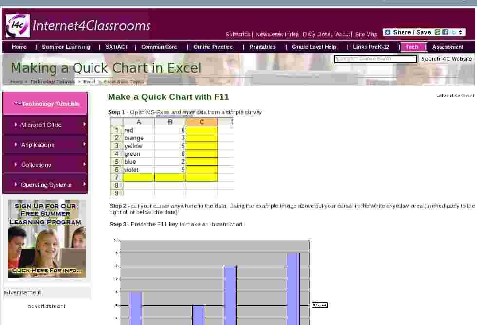
Make a Quick Chart with F11
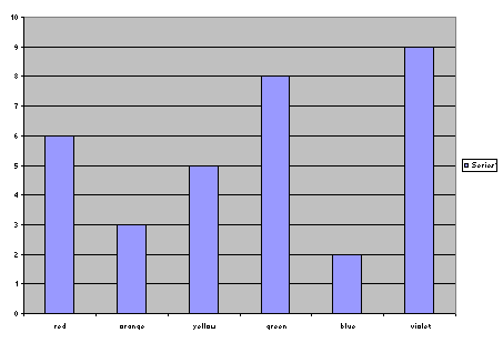
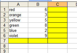
Step 1 - Open MS Excel and enter data from a simple survey
Step 2 - put your cursor anywhere in the data. Using the example image above put your cursor in the white or yellow area (immediately to the right of, or below, the data)
Step 3 - Press the F11 key to make an instant chart.
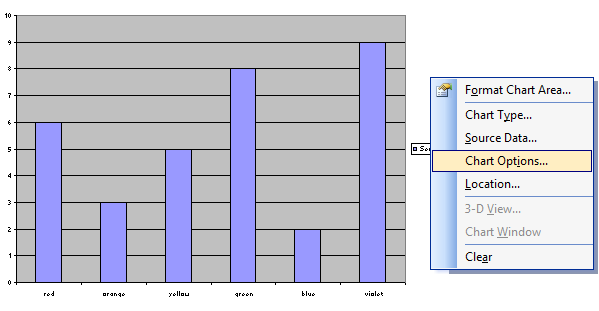
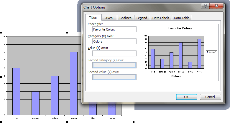
Step 4 - Add a title and names for x-axis and y-axis by right clicking in the white area surrounding the chart and selecting Chart Options.
Other changes could be made to the chart but this will let you begin using the chart with your class immediately.
If your cursor was anywhere else when you pressed the F11 key your chart will be nothing but a white sheet. F11 works just fine as long as the cursor is in the data or touching the data before you press the key.


Comments
Post a Comment